Student's t-Distribution (Continuous)
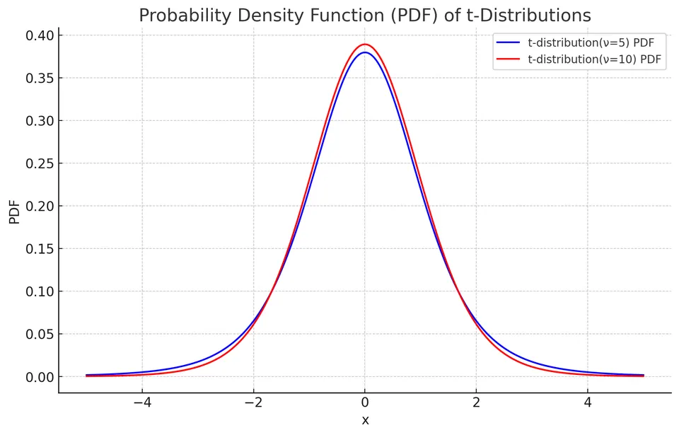
Student's t-distribution is a continuous probability distribution that arises when a normally distributed quantity is standardized using an estimated standard deviation rather than a known population standard deviation. Formally, if $Z\sim N(0,1)$ and $V\sim\chi^2(\nu)$ are independent, then $T=Z/\sqrt{V/\nu}\sim t(\nu)$. It has heavier tails than the normal distribution and approaches the normal distribution as its degrees of freedom increase. The t-distribution is denoted as $X \sim t(\nu)$, where $\nu$ is the number of degrees of freedom.
Probability Density Function (PDF)
The PDF of a t-distribution is given by:
$$f(x) = \frac{\Gamma\left(\frac{\nu + 1}{2}\right)}{\sqrt{\nu \pi} \, \Gamma\left(\frac{\nu}{2}\right)} \left(1 + \frac{x^2}{\nu}\right)^{-\frac{\nu + 1}{2}}$$
where $\Gamma(\cdot)$ is the gamma function.
Cumulative Distribution Function (CDF)
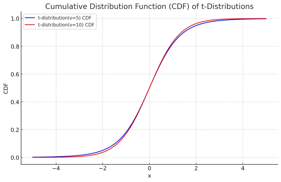
The CDF of a t-distribution can be expressed in terms of the regularized incomplete beta function $I_x(a,b)$. For $t\ne0$,
$$ F(t)=1-\tfrac12 I_{\frac{\nu}{t^2+\nu}}\!\left(\tfrac{\nu}{2},\tfrac12\right)\quad (t>0), $$
and $F(-t)=1-F(t)$ by symmetry.
Expected Value and Variance
The expected value (mean) of a t-distribution is equal to 0 for $\nu > 1$:
$$E[X] = 0$$
The variance of a t-distribution is given by:
$$\text{Var}(X) = \begin{cases} \frac{\nu}{\nu - 2}, & \text{if}\ \nu > 2 \\ \infty, & \text{if}\ 1 < \nu \le 2 \\ \text{undefined}, & \text{if}\ \nu \le 1 \end{cases} $$
Moments
The moment generating function of a t-distribution does not exist in a neighborhood of zero because of its heavy tails. Moments that do exist can be computed from the density.
- First Moment (Mean):
$$E[X] = 0, \text{ for } \nu > 1$$
- Second Raw Moment:
$$E[X^2] = \frac{\nu}{\nu - 2}, \text{ for } \nu > 2$$
Because the mean is zero, the second raw moment equals the variance whenever $\nu > 2$.
Example: Analyzing the Effect of Diet on Blood Pressure
A researcher investigates whether two diets lead to different average systolic blood pressure. The following data is collected from a random sample:
- Diet A: Sample size (n1) = 20, Mean (mean1) = 120, Standard Deviation (s1) = 8
- Diet B: Sample size (n2) = 25, Mean (mean2) = 130, Standard Deviation (s2) = 10
To compare the means, a two-sample t-test is employed.
I. Calculation of the T-statistic:
The t-statistic is calculated using the formula for Welch's two-sample t-test:
$$ t = \frac{(\text{mean1} - \text{mean2})}{\sqrt{(\text{s1}^2/\text{n1}) + (\text{s2}^2/\text{n2})}} $$
For the given data:
$$ t = \frac{(120 - 130)}{\sqrt{(8^2/20) + (10^2/25)}} \approx -3.73 $$
This value indicates the sample mean difference in units of its estimated standard error. With about 43 degrees of freedom the two-sided p-value is about $0.0006$, so the data are strong evidence of a difference in mean blood pressure.
II. Estimation of Degrees of Freedom:
The degrees of freedom can be estimated using the Welch-Satterthwaite equation:
$$ df \approx \frac{((\text{s1}^2/\text{n1}) + (\text{s2}^2/\text{n2}))^2}{(\text{s1}^4/(\text{n1}^2(\text{n1}-1)) + \text{s2}^4/(\text{n2}^2(\text{n2}-1)))} \approx 43.0 $$
These degrees of freedom are used to determine the reference t-distribution for the hypothesis test.
Applications
Student's t-distributions are widely used in hypothesis testing (such as the one-sample t-test, two-sample t-test, and paired t-test), confidence interval estimation for population means, and regression analysis when standard errors are estimated from data.