Backward Shift Operator

The symbol $B$ means “take the previous observation.” It acts on a sequence: $BX_t=X_{t-1}$, and applying it twice gives $B^2X_t=X_{t-2}$. It is useful because a long equation involving many lags can then be written as a polynomial acting on the whole sequence.

For example, $(1-B)X_t$ means the current observation minus the previous one. The 1 is the identity operator, which leaves the observation unchanged. Expanding the expression always returns an ordinary calculation with time-indexed values; there is no new source of randomness in the symbol $B$.

The same algebra connects AR dependence, MA shocks, and differencing. Moving AR lags to the left produces an AR polynomial, while collecting shock lags on the right produces an MA polynomial. Multiplying difference operators specifies several comparisons at once. Factoring a polynomial can reveal a unit root or a seasonal factor that is much harder to recognize in the expanded equation.

Worked calculation: differencing with the lag operator

For

$$ y_1,\ldots,y_5=8,\ 10,\ 13,\ 12,\ 15, $$

the backward shift gives $By_5=y_4=12$. Therefore,

$$ (1-B)y_5=y_5-y_4=15-12=3. $$

Applying the difference operator twice gives

$$ (1-B)^2y_5=y_5-2y_4+y_3=15-24+13=4. $$

The first difference is 3 because the level rises from 12 to 15. The second difference is 4 because that rise of 3 follows a fall of 1: the change in the changes is $3-(-1)$. Applying $1-B$ twice therefore does not mean subtracting the observation two periods ago. It gives the coefficients $1,-2,1$, as the expansion shows.

Definition and repeated shifts

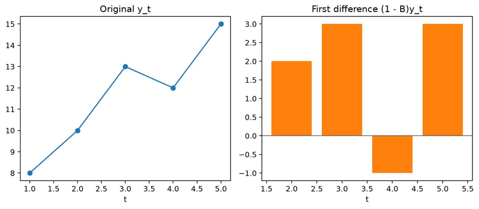
The backward shift operator, denoted by $B$, is a compact way to refer to earlier observations in a time series. It shifts the time index back by one period and simplifies the notation used in autoregressive, moving average, and mixed models.

For a time series $\{X_t\}$,

$$ BX_t=X_{t-1}. $$

Higher powers represent repeated shifts:

$$ B^2X_t=B(BX_t)=BX_{t-1}=X_{t-2}, $$

and, more generally,

$$ B^kX_t=X_{t-k}. $$

The operator acts on the sequence immediately to its right. In $B^2X_t$ it selects an observed value, while in $B^2Z_t$ it selects a shock. The multiplication rule $B^jB^k=B^{j+k}$ follows from performing one shift after another. Keeping the input sequence explicit avoids confusing an AR lag of an observation with an MA lag of an innovation.

Random Walk

Consider a simple random walk:

$$ X_t=X_{t-1}+Z_t, $$

where $Z_t$ is white noise. Because $X_{t-1}=BX_t$, the model can be written as

$$ X_t=BX_t+Z_t. $$

Rearranging gives

$$ (1-B)X_t=Z_t. $$

If we define

$$ \phi(B)=1-B, $$

then the random walk becomes

$$ \phi(B)X_t=Z_t. $$

The factor $1-B$ removes the accumulation that defines the random walk. It is called the first-difference operator because it changes the target from a level to a one-period increment. Its polynomial zero is 1, which explains the expression unit root. Unlike a stable causal AR polynomial, this factor cannot be inverted into a past-based filter with geometrically decaying coefficients.

Moving Average (MA) Process

Consider a moving average process of order 2, MA(2):

$$ X_t=Z_t+0.2Z_{t-1}+0.04Z_{t-2}. $$

Using $BZ_t=Z_{t-1}$ and $B^2Z_t=Z_{t-2}$,

$$ X_t=Z_t+0.2BZ_t+0.04B^2Z_t. $$

Factoring the noise sequence gives

$$ X_t=(1+0.2B+0.04B^2)Z_t. $$

Define

$$ \beta(B)=1+0.2B+0.04B^2. $$

Then the model is simply

$$ X_t=\beta(B)Z_t. $$

The polynomial $\beta(B)$ records the lag and coefficient of every shock entering the MA(2). Here its coefficient at lag zero is 1, followed by 0.2 at lag 1 and 0.04 at lag 2. Expanding the polynomial recovers the original equation, so the compact notation preserves the same model.

Autoregressive (AR) Process

Consider an autoregressive process of order 2, AR(2):

$$ X_t=0.2X_{t-1}+0.3X_{t-2}+Z_t. $$

Using the backward shift operator,

$$ X_t=0.2BX_t+0.3B^2X_t+Z_t. $$

Collecting all terms involving $X_t$ on the left gives

$$ (1-0.2B-0.3B^2)X_t=Z_t. $$

Define the AR polynomial as

$$ \phi(B)=1-0.2B-0.3B^2. $$

The process can then be written as

$$ \phi(B)X_t=Z_t. $$

The minus signs result from moving $0.2X_{t-1}$ and $0.3X_{t-2}$ from the right side to the left. The constant coefficient remains 1 because the current observation has coefficient 1. This bookkeeping matters when constructing software input: a model specified by AR coefficients $(0.2,0.3)$ can require the polynomial array $(1,-0.2,-0.3)$ rather than the coefficients as reported in the fitted equation.

Moving Average (MA) Process with a Constant Mean

An MA($q$) process with a constant term can be written as

$$ X_t=\mu+\beta_0Z_t+\beta_1Z_{t-1}+\dots+\beta_qZ_{t-q}. $$

Using the backward shift operator,

$$ X_t=\mu+\beta_0Z_t+\beta_1BZ_t+\dots+\beta_qB^qZ_t. $$

Factoring the shock sequence gives

$$ X_t=\mu+\beta(B)Z_t, $$

where

$$ \beta(B)=\beta_0+\beta_1B+\dots+\beta_qB^q. $$

Equivalently,

$$ X_t-\mu=\beta(B)Z_t. $$

The constant $\mu$ shifts the entire MA process by the same amount at every date. Since the shocks have mean zero, it is the process mean, not a trend slope. Subtracting it first produces a zero-mean equation to which the shock polynomial applies. In contrast, filtering a nonzero constant with an AR polynomial multiplies it by $\phi(1)$; this is why an AR intercept generally differs from the process mean.

Autoregressive (AR) Process of Order $p$

An autoregressive process of order $p$, AR($p$), is

$$ X_t=\phi_1X_{t-1}+\phi_2X_{t-2}+\dots+\phi_pX_{t-p}+Z_t. $$

Applying the backward shift notation,

$$ X_t=\phi_1BX_t+\phi_2B^2X_t+\dots+\phi_pB^pX_t+Z_t. $$

Rearranging gives

$$ (1-\phi_1B-\phi_2B^2-\dots-\phi_pB^p)X_t=Z_t. $$

With

$$ \phi(B)=1-\phi_1B-\phi_2B^2-\dots-\phi_pB^p, $$

the model becomes

$$ \phi(B)X_t=Z_t. $$

This compact form is useful because algebra on the polynomial $\phi(B)$ corresponds directly to algebra on the model's lag structure.

Combining operators without losing their interpretation

The backward shift operator is defined by

$$ BX_t=X_{t-1}. $$

It is algebraic shorthand, not a new random variable. For example,

$$ (1-B)y_t=y_t-y_{t-1}, $$

and

$$ (1-B)^2y_t=y_t-2y_{t-1}+y_{t-2}. $$

For $(y_3,y_4,y_5)=(13,12,15)$,

$$ (1-B)y_5=15-12=3, $$

and

$$ (1-B)^2y_5=15-2(12)+13=4. $$

The first expression measures a one-period change. The second measures the change in that change, so expanding the operator before interpreting it helps keep the calculation tied to the underlying observations.

Polynomial multiplication

Ordinary and seasonal differences combine as

$$ (1-B)(1-B^s)=1-B-B^s+B^{s+1}. $$

For $s=12$,

$$ (1-B)(1-B^{12})y_t=y_t-y_{t-1}-y_{t-12}+y_{t-13}. $$

The four terms compare a monthly change with the corresponding change one year earlier: $(y_t-y_{t-1})-(y_{t-12}-y_{t-13})$. The two operators commute for these constant-coefficient filters, so ordinary differencing followed by seasonal differencing gives the same interior values as the reverse order. Both calculations require observations through lag 13; the available sample must reflect that boundary requirement.

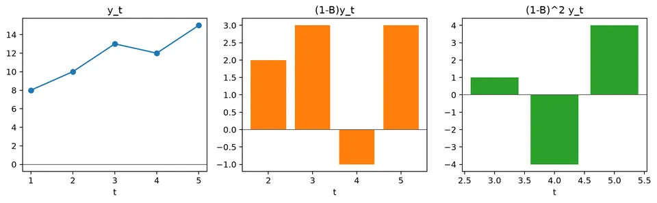
The figure shows the same idea geometrically: each operator selects lagged observations, and differencing combines those shifted values with positive and negative weights.

AR and MA polynomials

An AR(2) polynomial is

$$ \phi(B)=1-\phi_1B-\phi_2B^2. $$

An MA(2) polynomial under one common sign convention is

$$ \theta(B)=1+\theta_1B+\theta_2B^2. $$

The minus signs in the AR polynomial come from moving lagged observations to the left side of the equation. The plus signs in this MA polynomial follow the shock convention used here. Other texts use minus-signed MA coefficients, so compare the expanded equations before comparing parameter values or root calculations.

Implementation check

Check an implementation against a short sequence before fitting a model. Calculate one valid interior output by hand, write down its timestamp, and verify both its numerical value and its alignment with the software output. A first difference loses one starting observation; the combined monthly operator above needs 13 earlier observations. A correct set of numbers attached to the wrong dates is still an incorrect feature or forecast input.

Formula reference