Simple Linear Regression
Simple linear regression is a statistical method used to model the relationship between a single dependent variable and one independent variable. It aims to find the best-fitting straight line through the data points, which can be used to predict the dependent variable based on the independent variable.
In everyday terms, you can think of it as drawing a single straight line that best summarizes how one quantity (for instance, house price) tends to move whenever another quantity (such as house size) changes.
The Simple Linear Regression Model
The mathematical representation of the simple linear regression model is:
$$ y_i = \beta_0 + \beta_1 x_i + \varepsilon_i, \quad i = 1, 2, \dots, n $$
Where:
- $y_i$ is the $i$-th observation of the dependent variable.
- $x_i$ is the $i$-th observation of the independent variable.
- $\beta_0$ is the intercept (the expected value of $y$ when $x = 0$).
- $\beta_1$ is the slope (the average change in $y$ for a one-unit change in $x$).
- $\varepsilon_i$ is the error term, assumed to be independent with mean zero and constant variance $\sigma^2$.
The systematic part models $E[Y_i\mid x_i]=\beta_0+\beta_1x_i$. The error is the observation's deviation from that conditional mean and can include individual variation, omitted random influences, and measurement noise. A correctly specified mean model can still have nonzero errors: being correct about an average does not imply predicting every outcome exactly. After fitting, the residual is $e_i=y_i-\hat y_i$, which uses estimated rather than population coefficients.
Assumptions of the Model
For the simple linear regression model to be valid, several key assumptions must be met:
- Conditional mean: $E[\varepsilon_i\mid\mathbf X]=0$, where $\mathbf X$ denotes the predictor design. The linear expression describes the conditional mean, rather than requiring every point to lie on a line.
- Error dependence: the classical model assumes errors are independent, or uncorrelated for the Gauss-Markov variance result. Fitted residuals are generally correlated because they share estimated coefficients.
- Homoscedasticity: $\mathrm{Var}(\varepsilon_i\mid\mathbf X)=\sigma^2$ across observations. Heteroscedasticity changes the usual standard-error formula; it does not by itself prevent fitting least squares.
- Normal errors: conditional normality gives exact finite-sample t and F distributions. It is not required for computing least-squares coefficients.
- Predictor measurement: the interpretation assumes the recorded predictor is the intended quantity. Classical additive measurement error independent of the true predictor and model error attenuates the simple-regression slope toward zero. Other measurement-error mechanisms need not do so.
Normality is only needed for exact small-sample $t$ and $F$ inference; least squares itself needs only linearity, mean-zero errors, and (for the Gauss-Markov result) uncorrelated, equal-variance errors.
A quick way to remember these assumptions is “LINE” plus “no‐error-in-$x$”: Linearity, Independence, Normality, Equal variance. Diagnostic plots such as residual-vs-fit, Q-Q plots, and scale-location plots are routinely used to check whether LINE holds in practice.
Estimation of Coefficients Using the Least Squares Method
The goal is to find estimates $\hat{\beta}_0$ and $\hat{\beta}_1$ that minimize the sum of squared residuals (differences between observed and predicted values):
$\mathrm{SSE} = \sum_{i=1}^{n} (y_i - \hat{y}_i)^2$
$\mathrm{SSE} = \sum_{i=1}^{n} \bigl(y_i - \hat{\beta}_0 - \hat{\beta}_1 x_i\bigr)^2$
“Least squares” literally means “make the squares of the vertical distances from the data points to the line as small as possible.” Squaring the distances keeps positive and negative residuals from canceling and penalizes large misses more heavily than small ones, giving us a single objective function (SSE) to minimize.
Calculating the Slope ($\hat{\beta}_1$) and Intercept ($\hat{\beta}_0$)
The least squares estimates are calculated using the following formulas:
Slope ($\hat{\beta}_1$)
$$ \hat{\beta}_1 = \frac{S_{xy}}{S_{xx}} $$
$$ S_{xy} = \sum_{i=1}^n (x_i - \bar{x})(y_i - \bar{y}) $$
$$ S_{xx} = \sum_{i=1}^n (x_i - \bar{x})^2 $$
Equivalently, using sample covariance and variance (both with divisor $n-1$):
$$ \hat{\beta}_1 = \frac{\widehat{\mathrm{Cov}}(x, y)}{\widehat{\mathrm{Var}}(x)} = r_{xy}\,\frac{s_y}{s_x} $$
Intercept ($\hat{\beta}_0$)
$$ \hat{\beta}_0 = \bar{y} - \hat{\beta}_1 \bar{x} $$
Where:
- $\bar{x} = \dfrac{1}{n} \sum_{i=1}^{n} x_i$ is the mean of the independent variable.
- $\bar{y} = \dfrac{1}{n} \sum_{i=1}^{n} y_i$ is the mean of the dependent variable.
Notice how $\hat{\beta}_1$ is essentially the ratio of how $x$ and $y$ co-vary to how $x$ varies by itself. Intuitively, if $x$ and $y$ move together a lot compared with how much $x$ moves on its own, the slope must be steep; if they hardly move together, the slope must be shallow.
The coefficient formulas can be derived from the minimization. Differentiating SSE with respect to the intercept gives $\sum_i e_i=0$, hence $\hat\beta_0=\bar y-\hat\beta_1\bar x$. Substitution into the derivative for the slope gives $S_{xy}-\hat\beta_1S_{xx}=0$. A unique slope requires $S_{xx}>0$: if every predictor value is identical, the data cannot identify a change per unit of $x$.
The same normal equations give $\sum_i x_ie_i=0$. These are algebraic constraints on fitted residuals, not evidence that the unobserved errors are independent of the predictors in the population. A misspecified model can satisfy both equations in the training data.
Interpretation of the Coefficients
- The intercept ($\hat{\beta}_0$) represents the expected value of $y$ when $x = 0$, marking the point where the regression line intersects the $y$-axis.
- The slope ($\hat{\beta}_1$) indicates the average change in $y$ for each one-unit increase in $x$.
In some applications (for example, predicting salary from years of experience), $x = 0$ may not make practical sense. In such cases, $\hat{\beta}_0$ is still needed mathematically—even if we never literally interpret it—because it “anchors” the regression line.
Assessing the Fit of the Model
Total Sum of Squares (SST)
Measures the total variability in the dependent variable:
$$ \text{SST} = \sum_{i=1}^{n} (y_i - \bar{y})^2 $$
SST is what the variability looks like before we apply any model. It is the baseline against which every model is judged.
Regression Sum of Squares (SSR)
Measures the variability explained by the regression:
$$ \text{SSR} = \sum_{i=1}^{n} (\hat{y}_i - \bar{y})^2 $$
SSR tells us how much of the baseline variability SST our straight line succeeds in accounting for.
Sum of Squared Errors (SSE)
Measures the unexplained variability:
$$ \text{SSE} = \sum_{i=1}^{n} (y_i - \hat{y}_i)^2 $$
For an ordinary least-squares fit with an intercept, residuals are orthogonal to fitted values. Expanding $y_i-\bar y=(\hat y_i-\bar y)+e_i$ and summing squares therefore removes the cross term, giving $\mathrm{SST}=\mathrm{SSR}+\mathrm{SSE}$. A small SSE relative to SST indicates strong training fit; the identity and its interpretation should not be transferred automatically to held-out predictions or fits without an intercept.
Coefficient of Determination ($R^2$)
Indicates the proportion of variance in $y$ explained by $x$:
$$ R^2 = \frac{\text{SSR}}{\text{SST}} = 1 - \frac{\text{SSE}}{\text{SST}} $$
An $R^2$ value close to 1 suggests that the line captures most of the variability in the sample. In simple linear regression $R^2 = r_{xy}^2$, the squared sample correlation. A high $R^2$ does not by itself prove the relationship is linear or causal; always inspect residual plots.
For example, $R^2 = 0.87$ means “87 % of the variability in the outcome is captured by our one-predictor model,” leaving 13 % to chance, omitted variables, or measurement noise.
Hypothesis Testing
Testing the Significance of the Slope
- Null Hypothesis ($H_0$): $\beta_1 = 0$ (no linear relationship)
- Alternative Hypothesis ($H_a$): $\beta_1 \neq 0$
Test Statistic:
$$ t = \frac{\hat{\beta}_1}{\text{SE}(\hat{\beta}_1)} $$
Where:
$$ \mathrm{SE}(\hat\beta_1) = \frac{s}{\sqrt{\displaystyle\sum_{i=1}^n (x_i - \bar{x})^2}} $$
The intercept has standard error $\mathrm{SE}(\hat\beta_0) = s\sqrt{\dfrac{1}{n} + \dfrac{\bar{x}^2}{S_{xx}}}$, and a $(1-\alpha)$ confidence interval for the slope is $\hat\beta_1 \pm t_{1-\alpha/2,\,n-2}\,\mathrm{SE}(\hat\beta_1)$.
And the residual standard error is:
$$ s = \sqrt{\frac{\text{SSE}}{n - 2}} $$
Under $H_0$ and the model assumptions, the test statistic follows a $t$-distribution with $n - 2$ degrees of freedom.
A sufficiently large absolute t statistic gives a small two-sided p-value under the null reference, providing evidence that the population slope differs from zero under the model. Statistical detection does not establish practical importance or good prediction. An interval for $\beta_1$ shows the estimated association and its precision on the original units, while residual diagnostics and held-out evaluation address model adequacy and predictive value.
Example
Suppose we have the following data on the number of hours studied ($x$) and the test scores ($y$):
| Hours Studied ($x$) | Test Score ($y$) |
|---|---|
| 2 | 50 |
| 4 | 60 |
| 6 | 70 |
| 8 | 80 |
With only four paired observations this is a toy data set—perfect for hand calculations and for seeing each arithmetic step clearly, but obviously much smaller than what you would use in practice.
Step-by-Step Calculation
I. Calculate the Means
$$ \bar{x} = \frac{2 + 4 + 6 + 8}{4} = 5 $$
$$ \bar{y} = \frac{50 + 60 + 70 + 80}{4} = 65 $$
The means serve as the “balance points” of the $x$ and $y$ distributions. Centering each variable around its mean (by subtracting $\bar{x}$ or $\bar{y}$) makes the subsequent algebra cleaner and is the core of why the least-squares formulas work.
II. Compute the Sum of Squares and Cross-Products
Create a table to organize calculations:
| $x_i$ | $y_i$ | $x_i - \bar{x}$ | $y_i - \bar{y}$ | $(x_i - \bar{x})(y_i - \bar{y})$ | $(x_i - \bar{x})^2$ |
|---|---|---|---|---|---|
| 2 | 50 | -3 | -15 | 45 | 9 |
| 4 | 60 | -1 | -5 | 5 | 1 |
| 6 | 70 | 1 | 5 | 5 | 1 |
| 8 | 80 | 3 | 15 | 45 | 9 |
| Total | 100 | 20 |
Here, the cross-product column captures how $x$ and $y$ move together. Large positive numbers mean both variables are either above or below their means at the same time; large negative numbers would indicate opposite movements.
Sum of Cross-Products:
$$ \sum_{i=1}^{n} (x_i - \bar{x})(y_i - \bar{y}) = 100 $$
Sum of Squares of $x$:
$$ \sum_{i=1}^{n} (x_i - \bar{x})^2 = 20 $$
Think of the first sum as the numerator of the slope (how $x$ co-varies with $y$) and the second as the denominator (how much $x$ varies by itself).
III. Calculate the Slope ($\hat{\beta}_1$)
$$ \hat{\beta}_1 = \frac{\sum (x_i - \bar{x})(y_i - \bar{y})}{\sum (x_i - \bar{x})^2} = \frac{100}{20} = 5 $$
Interpreted literally, every additional hour of study is associated with a 5-point increase in the test score.
IV. Calculate the Intercept ($\hat{\beta}_0$)
$$ \hat{\beta}_0 = \bar{y} - \hat{\beta}_1 \bar{x} = 65 - (5)(5) = 40 $$
Although “0 hours studied” lies outside the observed data, the intercept mathematically pins down where the regression line crosses the $y$-axis.
V. Formulate the Regression Equation
$$ \hat{y} = 40 + 5x $$
This compact equation now lets us predict a test score for any study-hours value (within reason) by simple substitution.
VI. Predict the Test Scores and Calculate Residuals
| $x_i$ | $y_i$ | $\hat{y}_i = 40 + 5x_i$ | Residuals ($y_i - \hat{y}_i$) |
|---|---|---|---|
| 2 | 50 | 50 | 0 |
| 4 | 60 | 60 | 0 |
| 6 | 70 | 70 | 0 |
| 8 | 80 | 80 | 0 |
Every residual is exactly zero—an outcome that almost never occurs with real-world data and signals a perfect linear fit for these four points.
VII. Calculate the Sum of Squares
Total Sum of Squares (SST):
$$ \text{SST} = \sum (y_i - \bar{y})^2 = (-15)^2 + (-5)^2 + 5^2 + 15^2 = 500 $$
Sum of Squared Errors (SSE):
$$ \text{SSE} = \sum (y_i - \hat{y}_i)^2 = 0 $$
Regression Sum of Squares (SSR):
$$ \text{SSR} = \text{SST} - \text{SSE} = 500 - 0 = 500 $$
Since the regression explains all variability ($SSE = 0$), SSR equals SST, satisfying the identity $SST = SSR + SSE$.
VIII. Compute the Coefficient of Determination ($R^2$)
$$ R^2 = \frac{\text{SSR}}{\text{SST}} = \frac{500}{500} = 1 $$
An $R^2$ value of 1 indicates that the model perfectly explains the variability in the test scores.
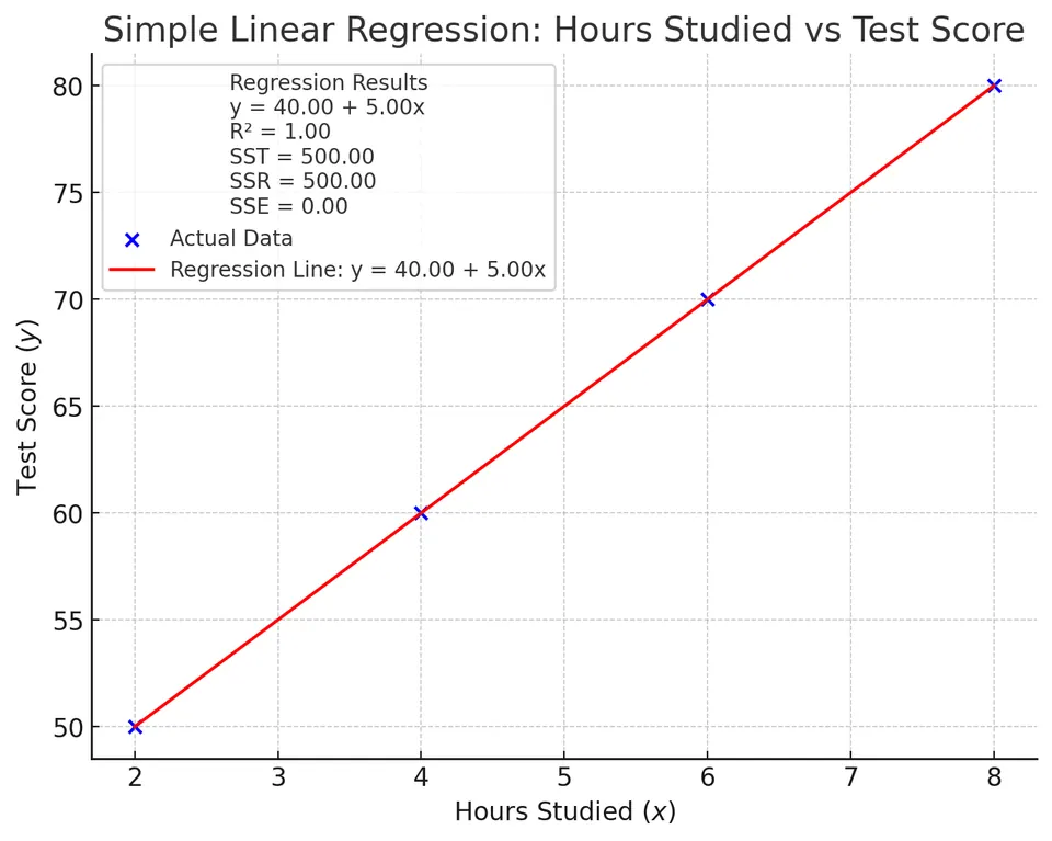
In practice you should be cautious: a perfect $R^2$ can be a sign of data entry errors, a derived variable (e.g. $y$ computed from $x$), or—more benignly—an extremely small, contrived sample like this one.
IX. Calculate the Standard Error of the Estimate ($s$)
$$ s = \sqrt{\frac{\text{SSE}}{n - 2}} = \sqrt{\frac{0}{2}} = 0 $$
The residual standard error measures typical residual size. Here, with all residuals exactly zero, the estimate collapses to zero as well.
The plug-in standard errors are therefore zero. This is a degenerate estimate of the noise scale, not evidence that the population coefficients are known with infinite precision. The four constructed points contain no residual information from which to estimate positive observation noise. The usual t ratio consequently has a zero denominator, so ordinary finite-sample inference cannot be justified from this example.
X. Hypothesis Testing (Optional)
In this case, the test statistic for $\hat{\beta}_1$ is undefined ($5/0$) because the standard error is zero. However, in practice, with more realistic data where $s > 0$, you would perform a $t$-test to assess the significance of the slope.
When $s$ is positive the $t$-test asks, “Is the observed slope big compared with the noise?” Here there is no noise, so the usual inferential machinery breaks down—which actually reinforces the lesson that perfect fits are the exception, not the rule.
For a new predictor value $x_0$, uncertainty in the fitted mean is proportional to $\sqrt{1/n+(x_0-\bar x)^2/S_{xx}}$. It is smallest near the center of the observed predictor values and grows with distance from that center. Prediction of an individual outcome adds observation noise as well. Far outside the observed range, uncertainty from a potentially wrong linear mean can dominate both calculations; the formula does not protect against extrapolation failure.