Simulations in Statistical Inference

Simulation approximates a probability calculation by repeatedly generating data under a specified mechanism. A parametric Monte Carlo experiment samples from an explicit model; a nonparametric bootstrap samples from the empirical distribution of the observed data; a permutation test rearranges data in a way justified by its null hypothesis. These procedures can estimate uncertainty when analytic calculations are difficult. They replace some algebra with computation, while retaining assumptions about the model, sampling units, and statistic.

Confidence Intervals for the Population Mean

Traditional Confidence Interval

For a population mean $\mu$, the traditional confidence interval is:

$$ \bar{x} \pm z_{1-\alpha/2} \cdot SE(\bar{x}) $$

where:

• $\bar{x}$: Sample mean.
• $z_{1-\alpha/2}$: Critical value from the standard normal distribution corresponding to the desired confidence level $(1 - \alpha)$.
• $SE(\bar{x})$: Standard error of the sample mean, typically estimated as $\frac{s}{\sqrt{n}}$ when the population standard deviation $\sigma$ is unknown. For small $n$ the critical value $t_{1-\alpha/2,n-1}$ is used instead of $z_{1-\alpha/2}$.

Limitations of Traditional Methods

• The normality assumption assumes that the sample mean $\bar{x}$ is normally distributed, which may not hold for small sample sizes or non-normal populations.
• Unknown standard error can be problematic when $SE(\hat{\theta})$ is difficult to compute due to complex estimators or unknown population parameters.

Simulations in Statistical Inference

Simulations approximate the sampling distribution of an estimator by reproducing a proposed data-generating or resampling process. The approximation is useful only to the extent that this process matches the inferential question. Generating more simulations reduces Monte Carlo error; it cannot compensate for a wrong model, a biased original sample, or an inappropriate independence assumption.

The Monte Carlo Method

The Monte Carlo method uses random sampling from a known distribution to approximate numerical results, particularly for estimating parameters and their variability.

Estimating an Unknown Parameter $\theta$

• The objective is to estimate a population parameter $\theta$, such as the average height in the U.S.
• The approach involves drawing $n$ observations, denoted as $X_1, X_2, \dots, X_n$, from the population.
• To estimate, compute the sample mean $\hat{\theta} = \bar{X}$.
• According to the law of large numbers, as $n$ increases, $\hat{\theta}$ will converge to the true population parameter $\theta$.

Estimating the Standard Error $SE(\hat{\theta})$

• The problem is that calculating the standard error $SE(\hat{\theta})$ analytically can be complex.
• A Monte Carlo solution involves drawing multiple independent samples to estimate $SE(\hat{\theta})$.
• Multiple samples are drawn, with $B$ independent samples of size $n$ from the population.
• For each sample $b$, compute estimates $\hat{\theta}_b$.
• The standard error is then estimated using the formula:

$$ SE(\hat{\theta}) \approx \sqrt{\frac{1}{B - 1} \sum_{b=1}^{B} (\hat{\theta}_b - \bar{\hat{\theta}})^2} $$

where $\bar{\hat{\theta}} = \frac{1}{B} \sum_{b=1}^{B} \hat{\theta}_b$.

Advantages

• The flexibility of this method allows it to be applied to complex estimators where analytical solutions are not feasible.
• Accuracy improves as the number of simulations $B$ increases.

Example: Estimating Standard Error Using Monte Carlo Simulation

In this example, we estimate the standard error of the sample mean $\hat{\theta}$ using a Monte Carlo approach. This method involves generating multiple independent samples from a population, calculating the mean $\hat{\theta}_b$ for each sample, and using these means to estimate the standard error.

Steps: - Draw $B$ independent samples of size $n$ from a normal population. - Calculate the sample mean $\hat{\theta}_b$ for each sample. - Estimate the standard error $SE(\hat{\theta})$ using the formula:

$$ SE(\hat{\theta}) \approx \sqrt{\frac{1}{B - 1} \sum_{b = 1}^{B} (\hat{\theta}_b - \bar{\theta})^2} $$

where $\bar{\theta} = \frac{1}{B} \sum_{b = 1}^{B} \hat{\theta}_b$ is the average of all sample means. For a normal population the exact value is $\sigma/\sqrt{n} = 15/\sqrt{30} \approx 2.739$.

Parameters:

• Population distribution: Normal with mean 100 and standard deviation 15.
• Sample size $n = 30$.
• Number of independent samples $B = 1000$.

Monte Carlo Simulation:

• Generate $B = 1000$ samples from a normal population with mean $100$ and standard deviation $15$.
• Each sample contains $n = 30$ values.
• For each sample, calculate the mean $\hat{\theta}_b$, and store these means in an array.

Estimate of Standard Error: - Calculate the overall mean of the sample means $\bar{\theta}$. - Use the formula for standard error estimation from the sample means.

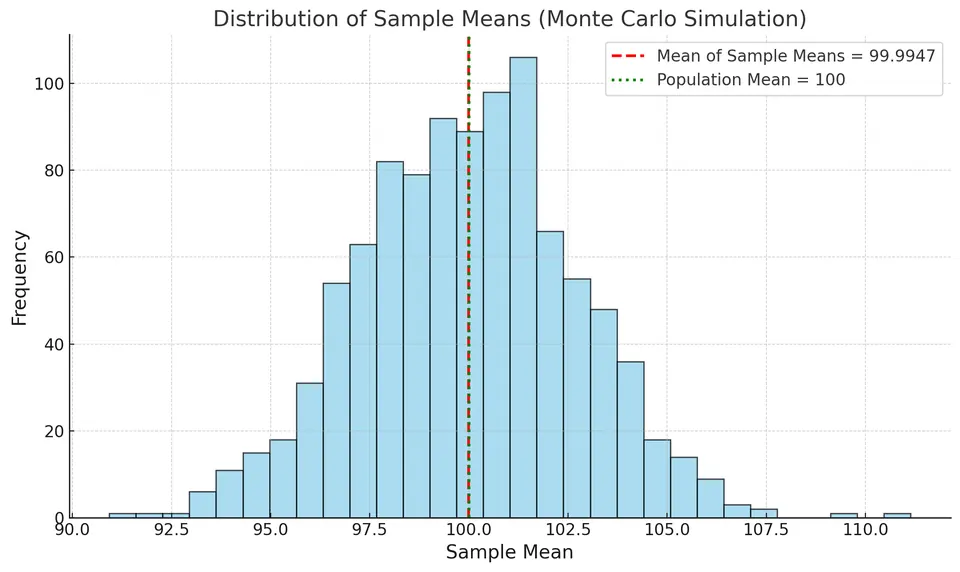
Estimated Standard Error (Monte Carlo): 2.7208

Here $n=30$ determines the true sampling spread $15/\sqrt{30}\approx2.739$. The number of repetitions $B=1,000$ determines how accurately the simulation estimates that spread. Increasing $B$ should stabilize the estimate around 2.739; it should not reduce the underlying standard error toward zero. The population model is known in this demonstration, whereas estimating its behavior from one real dataset requires an additional approximation.

The Bootstrap Principle

• The challenge arises when the population distribution is unknown, and only a single sample is available.
• The solution is to use the sample itself to approximate the sampling distribution of $\hat{\theta}$.

The Plug-in Principle

• The concept involves replacing the unknown population distribution with the empirical distribution derived from the sample.
• The justification is that if the sample is representative, its distribution closely approximates the population.

The empirical distribution puts mass $1/n$ at each observation. Drawing from it with replacement lets an observed value appear several times or not at all in a replicate. A bootstrap sample has $n$ draws, with an expected $n\{1-(1-1/n)^n\}$ distinct original indices, approximately $0.632n$ for large $n$. Sampling the same $n$ observations without replacement would merely reorder them and would give no bootstrap variation for an order-insensitive statistic such as the mean.

Bootstrap Procedure

1. Start with the original sample, denoted as $X = \{ X_1, X_2, \dots, X_n \}$.
2. Generate bootstrap samples by sampling with replacement from $X$ to create $B$ bootstrap samples $X^{*b}$, each of size $n$.
3. For each bootstrap sample $X^{*b}$, compute bootstrap estimates $\hat{\theta}^*_b$.
4. Finally, estimate the standard error using the formula:

$$ SE_{boot}(\hat{\theta}) = \sqrt{\frac{1}{B-1}\sum_{b=1}^{B}\left(\hat{\theta}^*_b - \bar{\hat{\theta}}^*\right)^2} $$

with

$$ \bar{\hat{\theta}}^* = \frac{1}{B}\sum_{b=1}^{B}\hat{\theta}^*_b. $$

Bootstrap Confidence Intervals

A bootstrap can approximate confidence intervals without a normal population model or an analytic standard-error formula. Validity still depends on the estimator and sampling structure. A statistic can have a poorly approximated bootstrap distribution near a boundary or with a tiny sample, and the ordinary empirical bootstrap can fail for quantities such as a sample maximum estimating a support endpoint. Interval choice should therefore be assessed rather than treated as automatic.

1. Normal Approximation Interval

• The assumption is that the sampling distribution of $\hat{\theta}$ is approximately normal.
• The interval is calculated as:

$$ [\hat{\theta} - z_{1-\alpha/2} \cdot SE_{\text{boot}}(\hat{\theta}), \quad \hat{\theta} + z_{1-\alpha/2} \cdot SE_{\text{boot}}(\hat{\theta})] $$

This approach is appropriate for symmetric distributions and large sample sizes.

2. Bootstrap Percentile Interval

• The concept of this interval relies on using percentiles from the bootstrap distribution.
• The interval is given by:

$$ [\hat{\theta}^*_{\alpha/2},\quad \hat{\theta}^*_{1-\alpha/2}] $$

• Here, $\hat{\theta}^*_{\alpha/2}$ represents the $100 \times (\alpha/2)$ percentile of the bootstrap estimates $\hat{\theta}^*_1,\dots,\hat{\theta}^*_B$.
• This method does not assume the distribution is normal.

3. Bootstrap Pivotal Interval

• This method (also called the basic bootstrap) reflects the bootstrap percentiles about $\hat{\theta}$, using the bootstrap distribution of $\hat{\theta}^*-\hat{\theta}$ to approximate that of $\hat{\theta}-\theta$.
• The interval is calculated as:

$$[2\hat{\theta} - \hat{\theta}^*_{1-\alpha/2},\quad 2\hat{\theta} - \hat{\theta}^*_{\alpha/2}]$$

Neither this interval nor the percentile interval is uniformly better; for skewed or biased statistics, bias-corrected variants such as BCa are often preferred.

For the basic interval, suppose bootstrap errors $\hat\theta^*-\hat\theta$ have quantiles $a$ and $b$ at $\alpha/2$ and $1-\alpha/2$. Approximate $P(a\leq\hat\theta-\theta\leq b)$ by $1-\alpha$, then solve for $\theta$ to get $[\hat\theta-b,\hat\theta-a]$. Substituting the bootstrap quantiles produces the reflected formula above. Unlike a percentile interval, this basic interval is not generally invariant to nonlinear transformations.

Bootstrapping for Regression

Bootstrapping can estimate the variability of regression coefficients when traditional assumptions (like normality of errors) may not hold.

Simple Linear Regression Model

$$ Y_i = a + b X_i + e_i, \quad i = 1, 2, \dots, n $$

• $Y_i$: Response variable.
• $X_i$: Predictor variable.
• $a$, $b$: Regression coefficients.
• $e_i$: Error terms, assumed to be independent with mean zero.

Residual Resampling

• The first step is to fit the original model and obtain estimates for $\hat{a}$ and $\hat{b}$.
• Next, compute the residuals as

$$ \hat{e}_i = Y_i - \hat{a} - \hat{b}\, X_i. $$

• Optionally, center the residuals to ensure they have a mean of zero.
• Then, bootstrap samples are created by resampling the residuals $\hat{e}_i^*$ with replacement and generating new responses as

$$ Y_i^* = \hat{a} + \hat{b}\, X_i + \hat{e}_i^*. $$

• Refit the model using the new responses to compute $\hat{a}^*$ and $\hat{b}^*$.
• Repeat this process for $B$ bootstrap samples to obtain a reliable estimate.
• Finally, estimate the variability by using the distribution of $\hat{b}^*$ to calculate $SE(\hat{b})$.
• This method assumes that the error terms $e_i$ are independent and identically distributed (in particular homoscedastic) and that the linear model is correctly specified.

Case Resampling (Pairs Method)

• Begin by bootstrapping samples by resampling the $(X_i, Y_i)$ pairs with replacement.
• Refit the model for each sample to calculate $\hat{a}^*$ and $\hat{b}^*$.
• Repeat this process for $B$ bootstrap samples.
• Estimate the variability by analyzing the distribution of $\hat{b}^*$ from the bootstrap results.
• An advantage of this method is that it captures the variability in both $X$ and $Y$ (a random-design view) and does not require homoscedastic errors.

Wild Bootstrap

• The purpose of the wild bootstrap is to handle heteroscedasticity, where the variance of the errors is not constant.
• The method involves multiplying residuals by random variables $\eta_i$ that have a mean of zero and a variance of one.
• New responses are then generated as

$$ Y_i^* = \hat{a} + \hat{b}\, X_i + \hat{e}_i\, \eta_i $$

to account for this variability.

Example: Estimating Variability of Regression Slope Using Residual Resampling

In this example, we demonstrate the Residual Resampling method to estimate the variability of the regression slope $b$.

Steps:

• Generate synthetic data with a known true intercept $a = 3$ and slope $b = 2$, along with random noise.
• Fit the original linear regression model and obtain estimates for $\hat{a}$ and $\hat{b}$.
• Compute the residuals

$$ \hat{e}_i = Y_i - \hat{a} - \hat{b}\, X_i. $$

• Perform bootstrapping by resampling the residuals, generating new responses, and refitting the model to obtain new estimates $\hat{a}^*$ and $\hat{b}^*$.
• Repeat the process for $B$ bootstrap samples to estimate the standard error of $\hat{b}$.

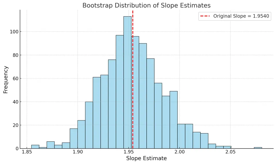
The initial linear regression model provided an estimate for the slope of approximately $\hat{b} = 1.954$.

Bootstrap Resampling:

• We performed $B = 1000$ bootstrap iterations by resampling the residuals from the original model and refitting the model to compute new slope estimates each time.
• This process generates a distribution of slope estimates under different bootstrap samples, reflecting the variability in the slope.
• The standard error of the slope was estimated to be 0.0312 (the classical OLS standard error is 0.0306), indicating the variability of the slope estimates.

Practical Considerations

Number of Bootstrap Samples $B$

• There is a trade-off between precision and computation: using a larger $B$ provides more precise estimates but increases computational demands.
• It is generally recommended to use at least $B = 1,000$ when calculating confidence intervals.

Assumptions and Limitations

• The bootstrap method relies on the sample being representative of the population for accurate results.
• Independence of observations is crucial, as the bootstrap assumes that each observation is independent of the others.
• Sample size can affect reliability, with the bootstrap being less dependable when dealing with very small samples.

Permutation Tests Approximate a Null Distribution

For two independent groups, consider the difference in sample means as a statistic. Under a null of identical distributions, labels are exchangeable conditional on the pooled observations. Rearrange the labels while retaining group sizes, recalculate the statistic, and compare the observed magnitude with the permuted magnitudes. In a randomized experiment, the assignment mechanism can instead justify a randomization test under an appropriate sharp null.

If $b$ out of $B$ randomly sampled null rearrangements are at least as extreme as the observation, a common valid Monte Carlo construction that includes the observed arrangement uses $(b+1)/(B+1)$. Reporting zero because no simulated value exceeded the statistic overstates the simulation's resolution. Paired data require within-pair exchanges or sign flips under suitable null symmetry or randomization assumptions; spatial or temporal dependence generally prevents arbitrary row shuffling.

Resample the Independent Unit

The ordinary row bootstrap assumes independently sampled units. Repeated measurements on a subject require a scheme that respects subjects, and serial dependence can require blocks. For regression, residual resampling conditions on the observed design and assumes a common error distribution; resampling pairs represents random design and can allow heteroscedasticity. A wild bootstrap preserves a residual scale at each design point but still needs an appropriate mean model and multiplier construction. Each method represents a different source of variation.