Geometric Distribution

The geometric distribution counts trials up to and including the first success. Unlike a binomial experiment, it does not fix the number of trials in advance. Repeat independent Bernoulli trials with a common success probability $p$ until the first success, and call its trial number $X$.

For $0<p<1$, write $X\sim\mathrm{Geometric}(p)$ with support $\{1,2,3,\ldots\}$. A different convention counts failures before the success. That variable is $Y=X-1$ and starts at 0. The shift changes the mean and event thresholds, so identify what is being counted before using a formula.

Probability mass function

For the first success to occur on trial $k$, the first $k-1$ trials must fail and trial $k$ must succeed. Independence gives

$$ P(X=k)=(1-p)^{k-1}p,\qquad k=1,2,3,\ldots. $$

There is no combinatorial multiplier: the success must be in the final position, and every preceding position is a failure. The masses form a geometric series whose total is $p/[1-(1-p)]=1$.

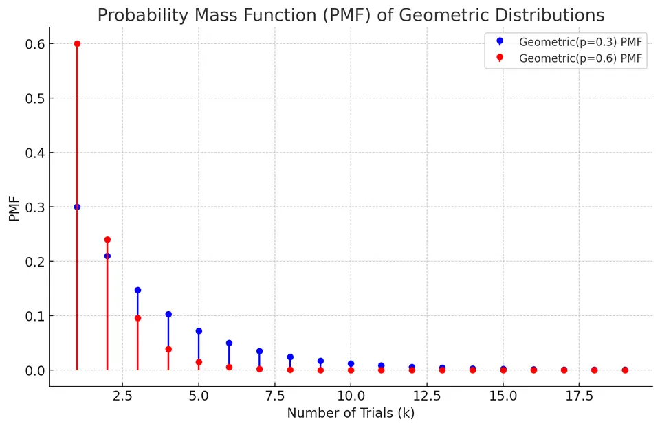
The probabilities decrease with $k$, but there is no finite maximum wait when $p<1$. A large wait is possible even when the expected wait is modest.

Cumulative and survival probabilities

The event $X>k$ means that the first $k$ trials all fail, giving $P(X>k)=(1-p)^k$. Taking its complement yields

$$ F(k)=P(X\le k)=1-(1-p)^k,\qquad k=0,1,2,\ldots. $$

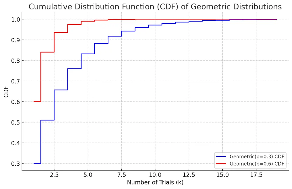
For a real threshold $x\ge1$, use $\lfloor x\rfloor$ in the integer formula; below 1 the CDF is zero. Distinguish $X>k$ from $X\ge k$: the latter requires only the first $k-1$ trials to fail.

The same tail formula shows memorylessness. After $m$ failures, the chance of waiting more than $k$ additional trials is

$$ P(X>m+k\mid X>m)=\frac{(1-p)^{m+k}}{(1-p)^m}=(1-p)^k. $$

The earlier failures do not change the future success probability under this model. That statement depends on independent trials with a constant $p$; it is not a claim that every repeated attempt in practice has no learning or deterioration.

Mean, variance, and MGF

The mean and variance under the total-trials convention are

$$ E[X]=\frac1p,\qquad \mathrm{Var}(X)=\frac{1-p}{p^2}. $$

The mean also follows from a restart argument: one trial is always needed; after a failure, the remaining wait has the original distribution. Thus $E[X]=1+(1-p)E[X]$.

Summing the exponential-weighted probability masses gives

$$ M_X(t)=\frac{pe^t}{1-(1-p)e^t},\qquad t<-\ln(1-p). $$

The bound is the convergence condition for the geometric series with ratio $(1-p)e^t$. Derivatives at zero give the raw moments, and subtracting the squared first moment from the second gives the variance. For the failures variable $Y$, $E[Y]=(1-p)/p$, while its variance is unchanged. At the boundary $p=1$, $X=1$ with probability 1 and its MGF is $e^t$ for every real $t$.

Example: flipping a fair coin

Let success mean heads and let $p=0.5$.

First head on the third flip

Only the pattern tails, tails, heads qualifies:

$$ P(X=3)=(1-0.5)^{3-1}(0.5)=0.125. $$

Expected number of flips

$$ E[X]=\frac1{0.5}=2. $$

This is a long-run average of first-head waiting times, not a guarantee of a head within two flips.

Variance of the wait

$$ \mathrm{Var}(X)=\frac{1-0.5}{0.5^2}=2. $$

The variance is in squared trials. The corresponding standard deviation is $\sqrt2$ trials.

Applications

Geometric waiting times model repeated independent attempts with a stable success chance, including certain inspection, packet-delivery, and reliability experiments. If attempts become easier after practice, harder after repeated damage, or dependent because of a changing environment, the constant-$p$ geometric mechanism needs to be reconsidered.

Practice: Exercises with worked solutions